Pathfinding Part 2 with A*
This is a continuation of our discussion on pathfinding. In the first part of our discussion, we investigated Dijkstra's algorithm. This time, we are digging into A* pathfinding.
Pathfinding, what is it
Quick research on pathfinding gives a plethora of resources discussing it. Pathfinding is calculating the shortest path through some 'network'. That network can be tiles on a game level, it could be roads across the country, it could be aisles and desks in an office, etc. etc.
Pathfinding is also an algorithm tool to calculate the shortest path through a graph network. A graph network is a series of nodes and edges to form a chart. For more information on this: click here.
For the sake of clarity, there are two algorithms we specifically dig into with this demonstration: Dijkstra's Algorithm and A*. We studied Dijkstra's Algorithm in Part 1.
A* Algorithm
A star is an algorithm for finding the shortest path through a graph that presents weighting (distances) between different nodes. The algorithm requires a starting node, and an ending node, and the algorithm uses a few metrics for each node to systematically find the shortest path. The properties of each node are fCost, gCost, and hCost. We will cover those in a bit.
Quick History
The A* algorithm was originated in its first state as a part of the Shakey project. That project was about designing a robot that could calculate its own path and own actions. In 1968, the first publishing of the A* project happened and it describes its initial heuristic function for calculating node costs.
A heuristic function is a logical means, not necessarily perfect means, of solving a problem in a pragmatic way.
Over the years the A* algorithm has been refined slightly to become more optimized.
Algorithm Walkthrough
Load the Graph
We first load our graph, understanding which nodes are clear to traverse, and which nodes are blocked. We also need to understand the starting node and ending node as well.
Cost the nodes
We first will assess the cost properties for each node. Cost is a term we are using that represents a distance between nodes. This will be a method that assigns the fCost, gCost, and hCost to each node.
Let's discuss these costs first. The costs are a weighting of each node with respect to its positioning between the starting and ending nodes.
The fCost of a tile is equal to the gCost plus the hCost. This is represented as such:
f=g+h
The gCost of the node is the distance cost between the current node and the starting node.
The hCost of the node is the 'theoretical' distance from the current node to the ending node. This is why we discussed heuristics earlier. This value is an estimate of the distance, a best guess. This makes guessing for a rectangular tilemap easy, since all tiles are distance 1 from each other in a grid, the method of guessing is just using the tile positions of the two nodes and using Pythagorean theorem to assess the distance. If the grid is irregular, some spatial data may need to be injected into the graphs creation to facilitate this heuristic, for example: x/y coordinate locations maybe.
Thus, the fCost is the sum of these two values. While simplistic, this is the value that is leveraged in the algorithm to determine the 'best' path.
Setup Buffers
After we've looped through all the nodes and costed them appropriately, we will utilize a buffer called openNodes. We will push the starting node into this, as it is the only node we 'know' about as of yet. We will use this openNodes buffer for much of the iterations we conduct in this algorithm.
We will leverage another buffer we will call either 'checked' or 'closed' buffer, and this is where the results of our algorithm will exist, as we process tiles from openNodes into this buffer.
Iteration
Then we get into the repeating part of the algorithm.
-
Look for the lowest F cost square in the open list. Make it the current square.
-
Move the current square to the closed buffer (list). Remove from openNodes, move to 'checked' nodes.
-
Check if the new current node is the endnode, this is the finishing condition. using the parent node properties of each node, walk backwards to the starting node, that's the shortest path
-
If not ending node, review all neighbor squares of current square, if a neighbor is not traversable, ignore it
-
Check each neighbor is in checked/closed list of nodes, if not, perform parent assignment, and add to open node list
This series continues to iterate while neighbors are being added to the open node list.
Example
Let's start with this example graph network.
We will manage our walkthrough with two different lists, open nodes and checked nodes. Black tiles above represent nodes that are not traversable. Let's define our start and stop nodes as indicated by the green S node and the blue E node.
The first step of A* algorithm is costing all the nodes, and let's see if we can show this easily.
For more clarity on the 'costing' step, let's talk through the core loop that is applied to each tile.
My process is to loop through each tile, and assuming it has either coordinates or and index, I can determine its distance from the start node and end node.
Let's do the first tile together. The first tile is coordinates (x:0, y:0), and the start node is coordinates (x: 1, y:1), while the end node is (x: 4,y:5). The gCost for this tile we can use Pythagorean theorem to calculate the distance as the hypotenuse.
js
js
This gives us a gCost of ~1.41.
We can repeat this equation for the hCost, but it is with respect to the end node coordinates.
js
js
This yields a hCost of ~6.40.
Knowing both now, we can determine the fCost of that node or tile, by adding the two together, making the fCost 7.82... with rounding.
We can repeat this process for each tile in the graph.
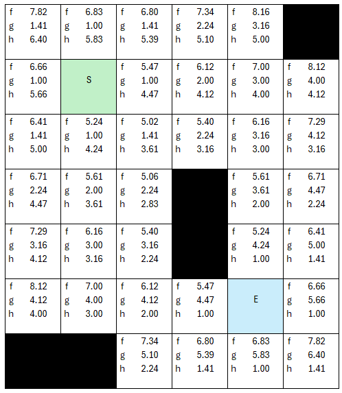
Why am I using floating point values here? There's a reason, if I simply use integers, then the distances wouldn't have enough resolution in digits, creating a little more unoptimized iterations, as the number of cells with equal f Costs would increase, here the fCosts are more absolute, and we will reduce the iterations. Simply put, if all the fCosts between 5.02 - 5.98 all are represented as 5 as an integer, it muddies up how the algorithm moves through and prioritizes the 'next' cell to visit. With floating points, this is explicit. Being a grid, all the distances are simple hypotenuse calculations using Pythagorean theorem.
Before we jump into the overall repetitive loop, we will add the startnode into our list of opennodes.
Now the algorithm can start to be repetitive. We set the startnode to the current node, and move it from open to checked lists.
We first check if our current node is the end node, which it is not, so we proceed.
The next step is to select the lowest fCost, and since the starting node is the only node in openlist, it gets selected, otherwise we would have selected randomly from the lowest value fCosts in the open node list. Now we look at all the neighbors. I will designate the pale yellow as our 'open node' list. We will use different colors for 'checked'.
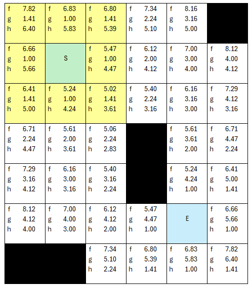
None are in the checked list, so we add them all to the opennodes list, and assign the current node as each nodes parent. To note, if a node is not traversable (black) then it gets ignored at this point, and not added to the list.
This then repeats as long as nodes are in the open node list, if we run out of open nodes without hitting the end node, then there's no path. When we hit the end node, we start building our return list by looping back through the parent nodes of each node. Starting at the end node, it will have a parent, that parent will have a parent... and so on until you hit the start node.
Let's walk through the example. Let's pick a tile with lowest f cost. As we select new 'current' nodes, we move that node to our checked list so it no longer is in the open node pool.
The lowest cost is 5.02, and grab its neighbors. Along the way we are assigning parent nodes, and adding the new neighbors to the openNodes list.
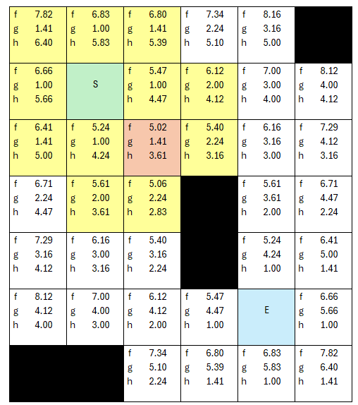
...but we keep selecting lowest cost node ( f cost of 5.06 is now the lowest to this point), we add neighers to opennodes, assign them parent nodes...
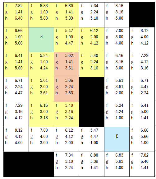
.. the next iteration, the fCost of 5.24 is now lowest, so it gets 'checked', and we grab its neighbors, assign parents..
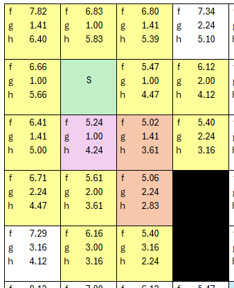
.. the next iteration, there are two nodes of 5.4 cost, so let's see how this CAN play out, and the algorithm starts to make sense at this point.
Let's pick the high road...
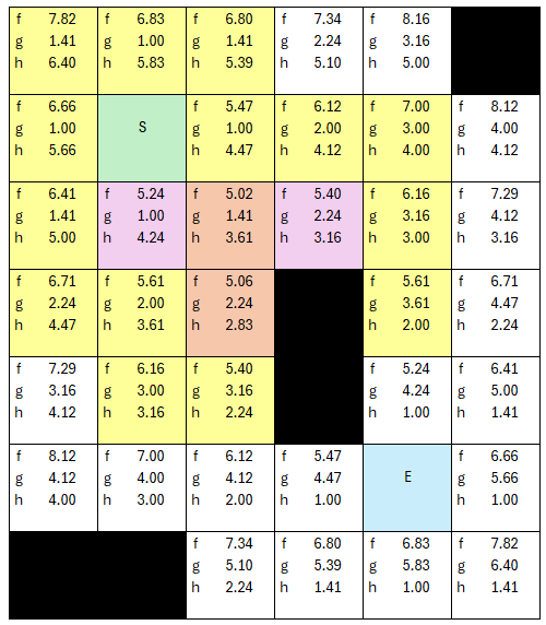
The new neighbors are assigned parents, and are added to the overall list of open nodes to assess. Which is the new lowest fCost now? 5.4 is still the lowest fCost.
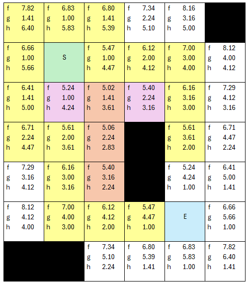
Yes, the algorithm went back to the other path and found a better next 'current' node in the list of open nodes. The process is almost complete. The next lowest fCost is 5.47, and there is more than one node with that value, so for the sake of being a completionist...
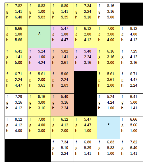
Still the lowest fCost is 5.47, so we select the next node, grab neighbors, assign parents... one thing I did differently on this table is showing the fCost of the ending node, which up till now wasn't necessary, but showing it here lets one understand how the overall algorithm loops, because the end node HAS to be selected as the next lowest cost node, because the check for end node is at the beginning of the iteration, not in the neighbor eveluation. So in this next loop, I don't make it yellow, but the end node is now been placed AS A NEIGHBOR into the list of open nodes for evaluation.
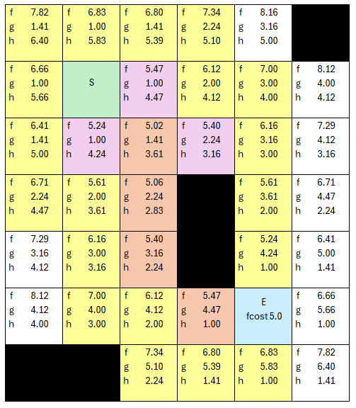
We now have our path, because the next iteration, the first thing we'll do is pick the lowest node fCost (5.0) and make it the current tile, and then test if it is the end node, which is true now.
We can return its path walking back all the parent node properties and see how we got there along the way.
The test
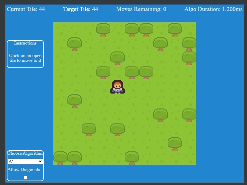
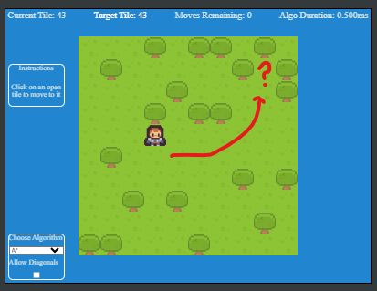
The demo is a simple example of using a Excalibur Tilemap and the pathfinding plugin. When the player clicks a tile that does NOT have a tree on it, the pathfinding algorithm selected is used to calculate the path. Displayed in the demo is the amount of tiles to traverse, and the overall duration of the process required to make the calculation.
Also included, are the ability to add diagonal traversals in the graph. Which simply modifies the graph created with extra edges added, please note, diagonal traversal is slightly more expensive than straight up/down, left/right traversal.
Why Excalibur
Small Plug...

ExcaliburJS is a friendly, TypeScript 2D game engine that can produce games for the web. It is free and open source (FOSS), well documented, and has a growing, healthy community of gamedevs working with it and supporting each other. There is a great discord channel for it HERE, for questions and inquiries. Check it out!!!
You can also find it on GitHub.
Conclusion
For this article, we briefly reviewed the history of the A* algorithm, we walked throught the steps of the algorithm, and then applied it to an example graph network.
This algorithm I have found is faster than Dijkstra's Algorithm, but it can be tricky if you're not using a nice grid layout. The trick comes into the 'guessing' heuristic of the distance between the current node and the endnode (hCost). If you using a grid, you can use the coordinates of each node and calculate the hypotenuse as the hCost. If it is an unorganized, non standard shaped graph network, this becomes trickier. For the moment, for the library I created, I am limiting A* to grid based tilemaps to make this much simpler. If the grid is not simple, I use Dijkstra's algorithm.
